When the first clients were introduced to our model, they saw the fit was so tight they nicknamed it the “glove.” Our model leverages cloud technology, which allows us to unleash tremendous computing power. This computing power allows us to discard the simplifying assumptions that were previously embedded in older models, freeing the data to speak for itself.

Risk Model Description

For single-name securities (Equities, ETFs, Mutual Funds), the model uses two sub-models to estimate risk: (i) a statistical model fitted to historical returns series (look-back), and (ii) a projection of potential future price movements based on the option implied volatility surface of that particular underlying security, where available.

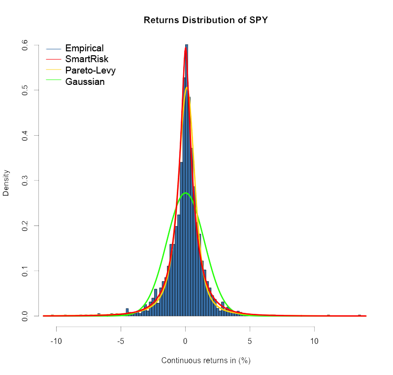
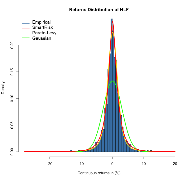
(i) The Historical Model: The workhorse statistical distribution used to model risk, whether for individual securities or portfolios is proprietary. In its simplest form, it is a three-parameter “heavy-tailed” distribution that has shown to provide overall superior fit to financial data (especially in the tails), compared to other well-known heavy-tailed candidates, such as the Student-t, Pareto-Levy, or GPD. As an illustration, we show the fit for the S&P500 ETF (SPY) and HerbaLife (HLF) below.

Acr7592112892928-2818729

Distribution-of-HLF copy


(ii) The Implied Volatility-Based Model: This model is proprietary as well. It is based on a study of every option traded in the US since 2002, and projects a distribution of future returns based on today’s implied volatility surface.

For the two symbols above, we can compute Expected Tail Loss (ETL) using both the historical and IV-based methods. Results for the 99.5% confidence interval are presented in the table below:

Symbol  Bearish Historical  Bullish Historical  Bearish IV-Based  Bullish IV-Based
 SPY  -8.81%  9.69%  -4.49%  4.94%
HLF  -14.56%  17.15%  20.17% 24.46%


Note on the Treatment of Option Positions

Because option prices are non-linear functions of their underlying prices, one cannot simply use their historical prices to calculate a historical returns time series.

Instead, for each option, the model (i) first calculates the vector of theoretical option prices for each date using the price of the underlying security for that particular date, keeping the same moneyness, time to maturity, implied volatility, interest rate and dividend rate as of the most recent value.

Then, (ii) for each date in the time series vector, the model calculates theoretical option prices k-period ahead using the corresponding underlying prices, and by decreasing the time-to-maturity by k periods.

The historical returns series for an option contract is then simply obtained by computing the discrete returns between the prices obtained in step (i) and step (ii)... to continue reading, download the full white paper.

Download